

Scrutinizing Stock Prices in Eye of Benford’s Law Using Python

The Law
One and half decade back while I was pursuing my Chartered Accountancy, I had come across interesting topic on fraud detection in accounting and taxation, using Benford’s Law. Benford’s Law is nothing complex, it just states that unless any data is manipulated, the occurrence of first digit of naturally occurring numbers follows a pattern and shows consistent probability of occurrence. This is because of simple logic that the first digit if it is 1 must increase by 100 percent to change to 2 while for 2 to change to 3, it only needs to increase by 50 percent. Newcomb first noticed and Frank Benford rediscovered this occurrence of logarithmically decaying distribution of first digit from 1 to 9 represented by the formula.
P(D1=d) = log10(1 + 1/d) (Where d is the number from 1 to 9)
Being in a role of Investment Banker at present, I wondered whether the often controversy of anomalies in the trading of stock in market could be scrutinized using same law. While there seemed difficulty as for Benford’s Law to hold true, there needs to be large sample size, but manipulations or malpractices in any trading stock happens for a short period. However, few have tried to scrutinize the rampant trading manipulations of cryptos like Bitcoin. This law however has been effectively used in fraud detection in accountancy, taxation, elections etc.
Dataset
For veracity of whether the Benford’s Law applies truly, I took the NEPSE Closing prices from the inception. Further data of closing prices of two highly volatile scrips from Finance Companies Sector was taken for testing purpose.
Python Codes
Step 1-Import necessary Python Libraries and Defining Benford’s Percentages
#Importing required Libraries
import numpy as np
import pandas as pd
import collections
import matplotlib.pyplot as plt
#Probabilities as per Benford’s Law
benfords_prob = [30.1, 17.6, 12.5, 9.7, 7.9, 6.7, 5.8, 5.1, 4.6]
Step 2-Import NEPSE Closing Indexes and Sample Finance Company Prices
#Reading closing index of NEPSE
NEPSE_data = pd.read_csv("NEPSE.csv")
NEPSE_close=NEPSE_data["Close"]
#Reading prices of sample Finance Company No. 1
F01_data = pd.read_csv("F01.csv")
F01_data.columns = "Date","Prices"
F01_prices=F01_data["Prices"]
#Reading prices of sample Finance Company No. 1
F02_data = pd.read_csv("F02.csv")
F02_data.columns = "Date","Prices"
F02_prices=F02_data["Prices"]
Step 3-Creating Function for the purpose of calculating percentage
#Function to calculate percentage of first digit occurrences
def calc_percentage(data):
first_digit_percentage = [] #Defining List to accumulate values
first_digits = list(map(lambda n: str(n)[0], data))
first_digit_frequencies = collections.Counter(first_digits)
for n in range(1, 10):
data_frequency = first_digit_frequencies [str(n)]
data_frequency_percent = (data_frequency / len(data))*100
first_digit_percentage.append(data_frequency_percent)
return (first_digit_percentage)
Outcomes (Visualization)
Step-4 Plotting and Visualizing the Graphs
#Calculating first digit of NEPSE closing prices and plotting using Matplotlib alongside Benford’s line
x=np.arange(1,10)
y=calc_percentage(NEPSE_close)
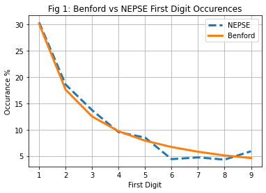
plt.title("Fig 1: Benford vs NEPSE First Digit Occurences")
plt.xlabel("First Digit")
plt.ylabel("Occurance %")
plt.plot(x,y,label='NEPSE',linewidth=3,linestyle="dashed")
plt.plot(x,benfords_prob,label='Benford',linewidth=3,linestyle="solid")
plt.grid()
plt.legend()
#Calculating first digit of Sample Finance Co # 1 Prices and plotting using Matplotlib alongside Benford’s line
x=np.arange(1,10)
y=calc_percentage(F01_prices)
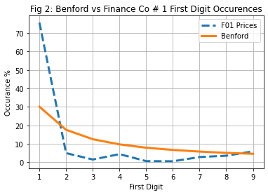
plt.title("Fig 2: Benford vs Finance Co # 1 First Digit Occurrences")
plt.xlabel("First Digit")
plt.ylabel("Occurance %")
plt.plot(x,y,label='F01 Prices',linewidth=3,linestyle="dashed")
plt.plot(x,benfords_prob,label='Benford',linewidth=3,linestyle="solid")
plt.grid()
plt.legend()
#Calculating first digit of Sample Finance Co # 2 Prices and plotting using Matplotlib alongside Benford's line
x=np.arange(1,10)
y=calc_percentage(F02_prices)
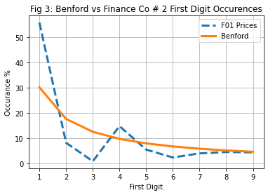
plt.title("Fig 3: Benford vs Finance Co # 2 First Digit Occurrences")
plt.xlabel("First Digit")
plt.ylabel("Occurance %")
plt.plot(x,y,label='F01 Prices',linewidth=3,linestyle="dashed")
plt.plot(x,benfords_prob,label='Benford',linewidth=3,linestyle="solid")
plt.grid()
plt.legend()
Conclusions:
While as initially disclaimed, Benford’s law can not be litmus test for finding manipulations, but given that there is adequately large data, the prescribed probability distribution of Benford’s Law should certainly hold true if it is naturally occurring data. In Figure No. 1 when NEPSE Closing Indexes are plotted over Benford’s distribution, the plots seem to be nearly overlapping each other except at digit 6 and 7. Indexes which are mix of large number of various scrips can hardly be manipulated in huge amount and hence seems to follow the Law. In case of sample Finance Companies which had largely volatile price movements in recent periods, the plot seemed hugely deviating from the Law specially where the first digit is 1 (so possibly somebody wanted to keep prices above 1000 😉)
CA. Dinesh Thakali (Author is employee of Prabhu Bank Ltd and currently Managing Director at Prabhu Capital Ltd. Views expressed are personal and Author intends only to illustrate the results of Law but doesn’t prescribes or authenticates usage of the methods for any purpose) —Published in ShareSansar.com — 2022-April-18